Publication: Cheng‑Yu Tsai, Suwan Kim, Sung‑Kyu Lim. “Capacitance Extraction via Machine Learning with Application to Interconnect Geometry Exploration”. IEEE/ACM International Conference on Computer‑Aided Design (ICCAD) 2025
- Motivation
- Contributions
- Background
- Approach Overview
- Pattern Extraction Algorithm
- Feature Representation
- Machine Learning Strategy
- Netlist Generation
- Experimental Results
- Conclusion
Motivation
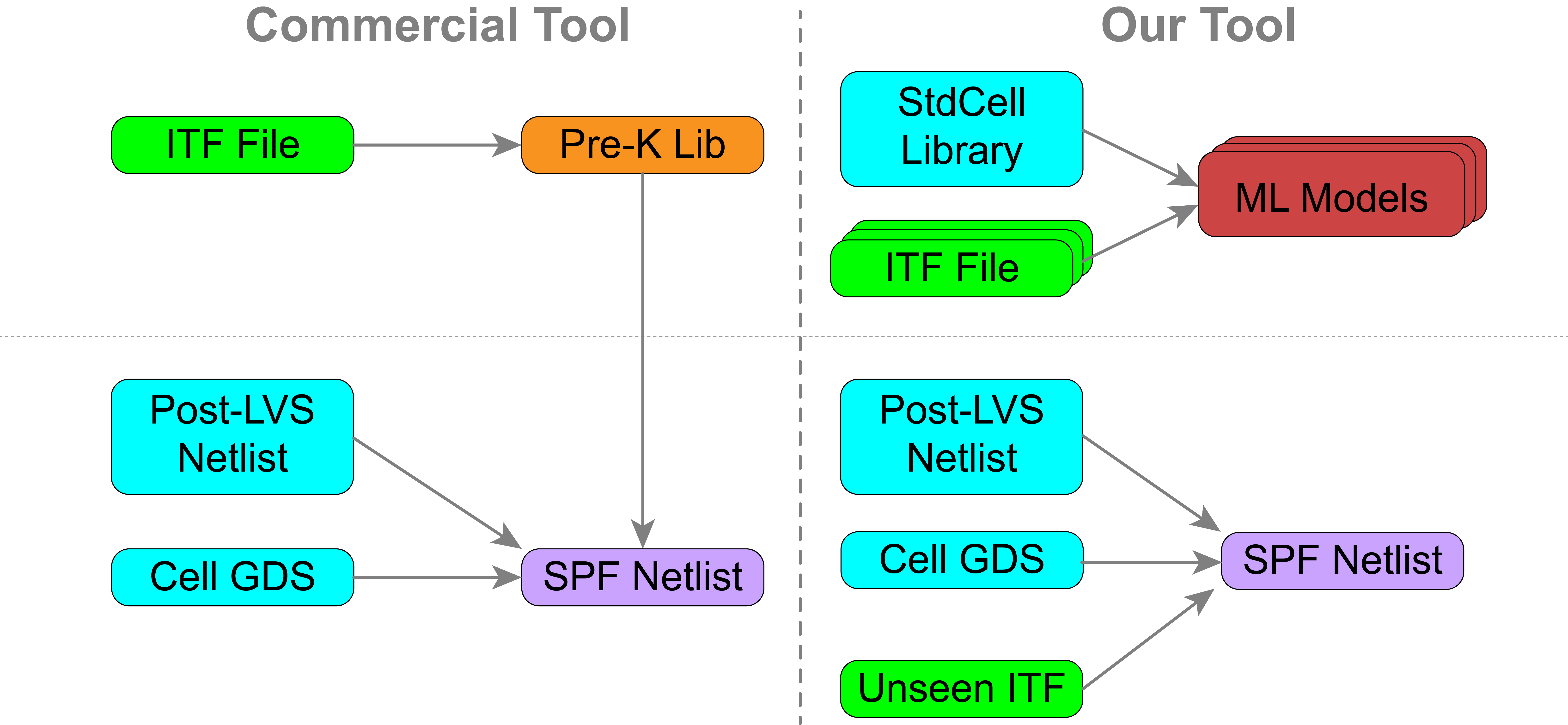
As transistors shrink, parasitic resistance and capacitance (R/C) dominate chip delay and power. Commercial extraction tools (e.g., Synopsys StarRC, Cadence QRC, Siemens xACT) face two main problems:
- Slow response to process changes – e.g., re-generating a netlist for a thickness change can take 25 minutes to days.
- Pattern mismatch – pre-characterized libraries are generated without real layouts, causing significant errors.
The proposed method leverages machine learning (ML) to:
- Encode multiple interconnect technology files (ITFs) into ML models (avoiding pre-characterization).
- Extract patterns directly from layouts to minimize mismatch.
- Generate R/C netlists faster and more accurately.
Contributions
- 2.5D R/C extraction algorithm: From pattern extraction to netlist generation.
- Layer thickness encoding: Enables interpolation/extrapolation of unseen thicknesses.
- Model choice: Compared DNN vs. LightGBM (LGB is ~10× faster, suffices in most cases).
- Via awareness: Demonstrated vias contribute 7-11% of total capacitance.
- Accuracy: Achieved within ±4% error compared to field solver, far better than conventional tools.
Background
Traditional Flow
Pattern-based (2.5D) extraction involves:
- Pre-characterization: Generate 2D patterns, solve with field solver, build lookup tables.
- Extraction: Slice layouts, match patterns, assemble parasitic netlist.
Limitations:
- Pre-characterization is slow and not layout-aware.
- Manual pattern selection and curve fitting require expertise.
ML Opportunity
Pattern extraction and regression can be reformulated as a supervised learning problem:
- Input: Shape coordinates → feature vectors.
- Output: Capacitances computed by field solver.
- Model: ML learns the mapping automatically, generalizes across unseen thicknesses.
Approach Overview
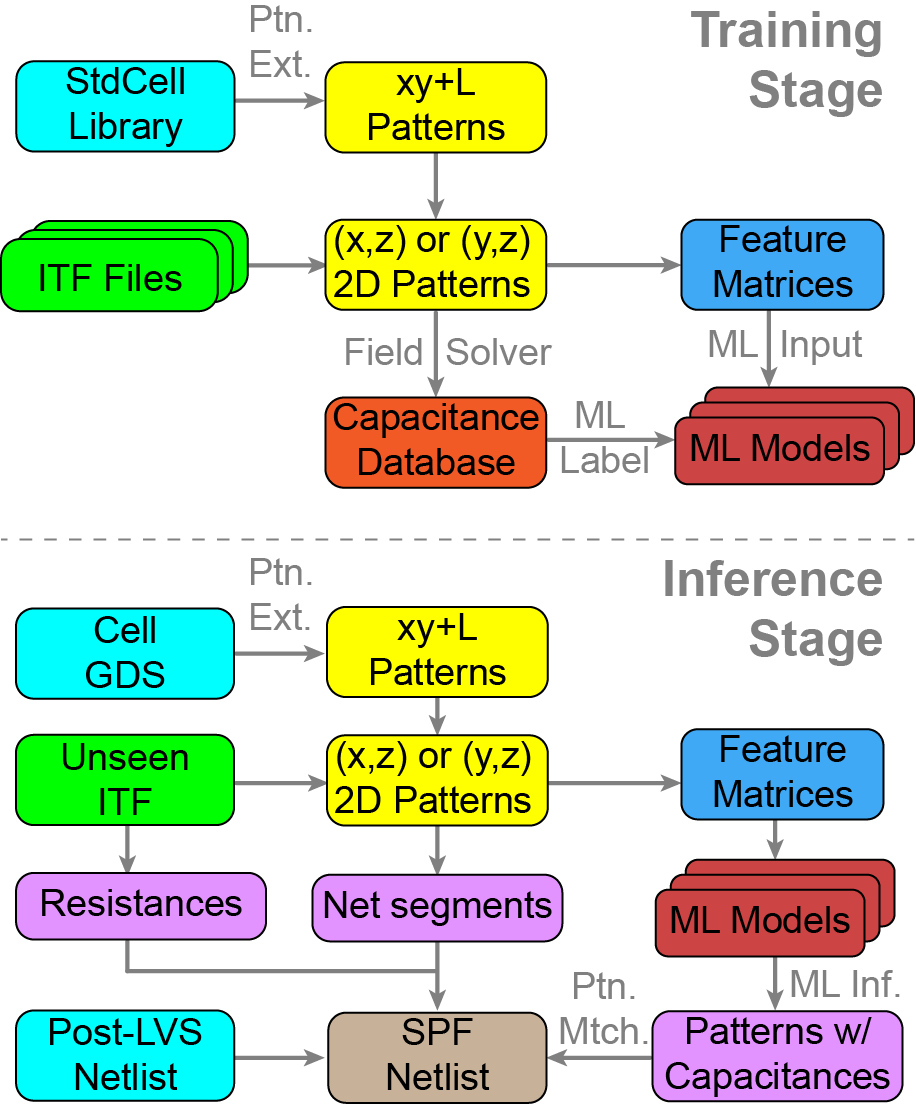
Figure: Training and inference stages.
- Training stage
- Extract cross-section patterns from layouts (GDS).
- Map to ITF-derived z-coordinates.
- Solve patterns with 2D field solver (Raphael) to generate capacitance labels.
- Encode as feature matrices and train ML models.
- Inference stage
- Extract patterns from new GDS.
- Predict capacitances using trained ML models.
- Match patterns to layout locations.
- Generate parasitic netlist with both resistances and capacitances.
Pattern Extraction Algorithm
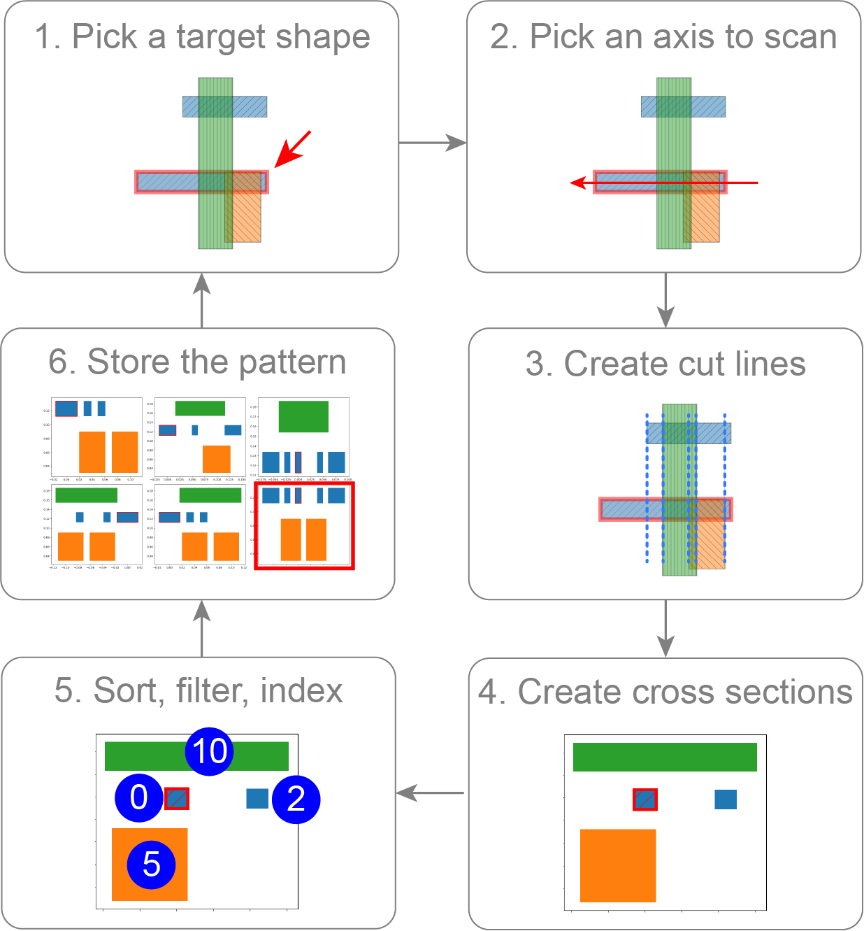
Figure: Steps of the extraction algorithm.
Steps:
- Pick a target shape (aggressor).
- Scan along x and y directions.
- Create cut lines at neighbor boundaries.
- Collect victims overlapping segments → cross-section patterns.
- Apply sorting, filtering, and indexing for ML-ready structure.
Key Policies
- Sorting: Organize shapes by relative position.
- Filtering: Keep up to two nearest shapes per direction; discard negligible contributors.
- Indexing: Assign consistent slots to aggressor/victims for feature vector translation.
Feature Representation
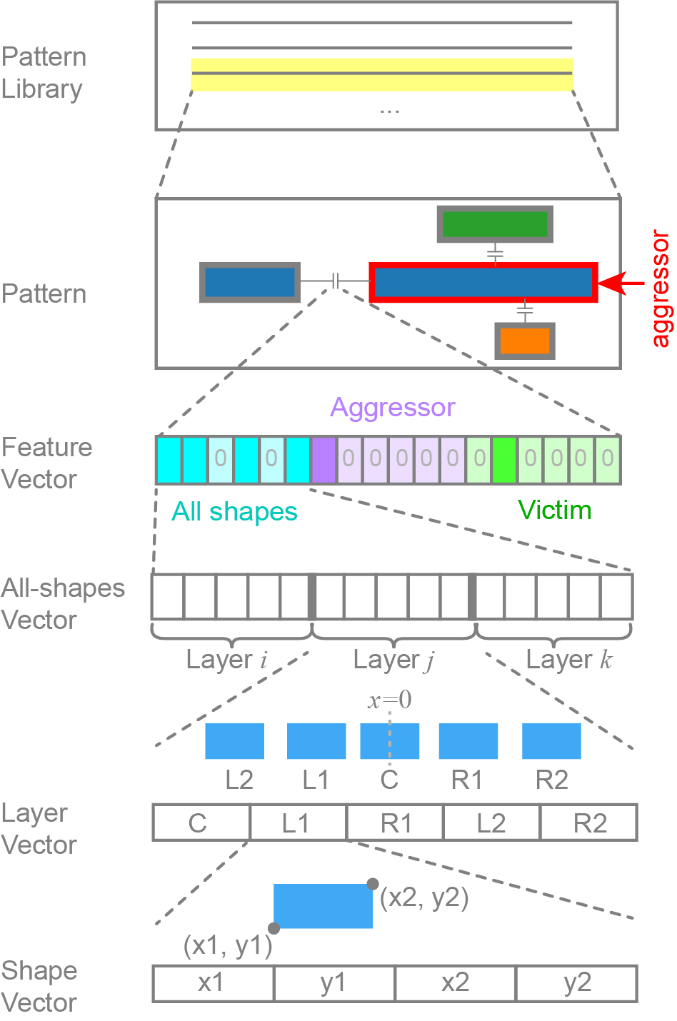
Figure: Hierarchical breakdown of the feature vector.
- All-shapes vector: Encodes geometry of up to 15 shapes (five per layer).
- Aggressor vector: Copy with only aggressor retained.
- Victim vector: Copy with only victim retained.
- Final feature vector: Concatenation of all three (dimension ≤ 300).
Preprocessing:
- Data cleaning: Remove shielded, negligible capacitances.
- Scaling: Normalize capacitances (\(10^{-16}\) to \(10^{-18}\) F/µm) to \([0,1]\).
- Augmentation: Horizontal flips increase dataset diversity.
Machine Learning Strategy
- Model separation: Train one model per layer combination (12 models total for test PDK).
- Model choice:
- Use LightGBM for most cases (fast, accurate for low-sensitivity capacitances).
- Use DNN for high-sensitivity cases (e.g., lateral capacitances).
- Training:
- Hyperparameters tuned with Optuna.
- DNN: 2000 epochs; LGB: 2000 iterations.
- Training time: ~2.5 days single machine, 1 day with parallelization.
Netlist Generation
- Subnode creation: Divide nets into smaller segments (breakpoints for resistors/capacitors).
- Merging reciprocal capacitances: Ensure aggressor/victim pairs are stored once.
- Subnode reduction: Collapse excessive nodes into mandatory ones (boundaries, vias, pins).
- Resistance modeling: Compute conductor resistance (ρ·l/wt) and via resistance (RPV).
Experimental Results
Setup
- PDK: imec N2 nanosheet predictive PDK.
- Library: 94 standard cells.
- Patterns: ~33k unique patterns, 2.3M total data points.
- Process parameter varied: M0 thickness (22–58 nm training, 18–62 nm testing).
Results
- Accuracy:
- >75% of predictions within ±1% error across thicknesses (except margins).
- With vias: error within ±2% delay, ±6% capacitance; without vias: up to -11% error. → Vias cannot be omitted.
- Speed:
- Per-pattern: field solver 300 ms vs. LightGBM 5 ms vs. DNN 50 ms.
- Cell-level: 8x - 14x speedup over StarRC FS.
- No pre-characterization needed (saves 5-25 minutes).
- Cell-level comparison:
- Total capacitance: Within ±6% vs. field solver.
- Delay: Within ±2%.
- StarRC (pattern-based) suffers -35% to -45% error in capacitance.
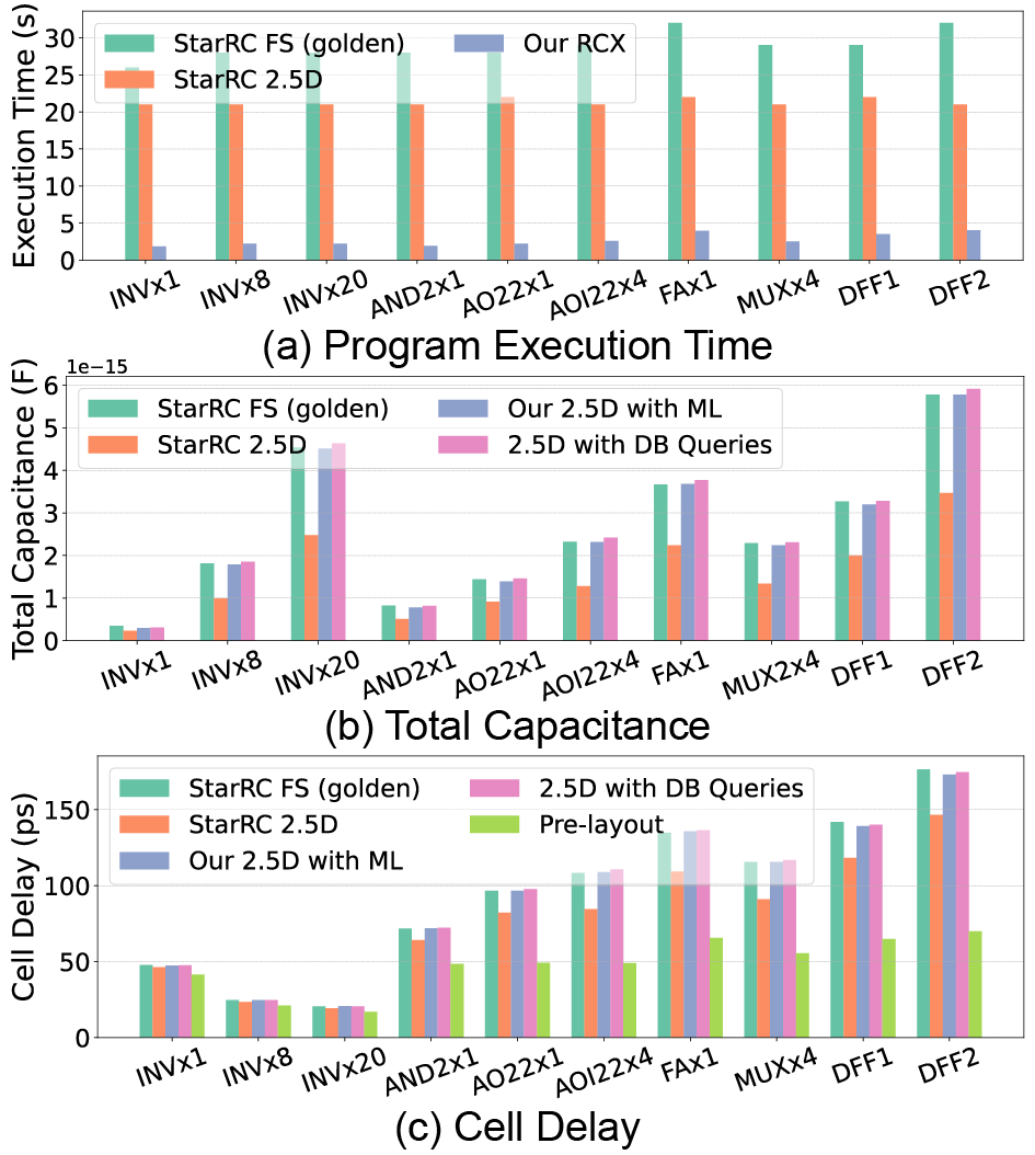
Figure: Cell-level comparison of capacitance and delay.
Conclusion
This work demonstrates that machine learning can accelerate parasitic extraction 8x-14x while maintaining accuracy within ±6%. Key findings:
- Automatic pattern extraction for pre-characterization is essential. Not using real layout in pre-characterization introduces up to 45% error.
- Via inclusion is essential (ignoring them induces up to 11% error).
- 2.5D pattern-based extraction has untapped potential when combined with ML.
- Regression accuracy is the bottleneck—future work should push toward better ML models.
Takeaway: ML-enabled parasitic extraction offers a promising direction for design-technology co-optimization (DTCO) by enabling fast, accurate exploration of process parameters.